Due on F̶e̶b̶ ̶2̶7̶ M̶a̶r̶c̶h̶ ̶6̶ March 10

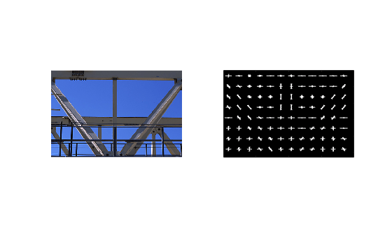
• In this HW, you are asked to implement histogram of oriented gradient (HOG) descriptor as discussed in class. HOG is not just used in interest point descriptors such as SIFT. It is also a widely used feature for object recognition.

• For simplicity, we will ignore the step of finding interest points but simply partition the image into cell/patch and compute the HOG in each cell.

  • Basically within in cell, you should compute the gradient for each pixel and convert it to polar coordinate (rho and theta).

  • You should then quantize theta into a fixed number of bins. (Be careful that 1 and 359 degrees probably should belong to the same bin.)

  • Add rho of each pixel to the corresponding bins. For example, say we have 4 bins: bin 1 \(\leftarrow [-45^o,45^o)\), bin 2 \(\leftarrow [45^o,135^o)\), bin 3 \(\leftarrow [135^o, 225^o)\), and bin 4 \(\leftarrow [225^o, 315^o)\). Now, gradients of the first 4 pixels in the patch are \((2,25^o), (4,-10^o), (0.1,100^o),\) and \((1,90^o)\). Note that the first two pixels belong to bin 1 and the next two belong to bin 2. So just from the contribution of these four pixels. The histogram representation for this patch should be \([2+4,0.1+1,0,0]=[6,1.1,0,0]\).

• You should test on the gantrycrane image. It is also available in the zip package. You can use either matlab or opencv-python as usual. However, I have written a file to display the result in matlab. If you would like to test the code with my file, you can first export your hog result to a mat file using scipy.io.savemat. I have already store the result in a mat file and you may run test_your_hog.m to preview the result. (Note that the Matlab demo appears to display the gradient with \(90^o\) rotation and thus shows something a bit difference.)

• Besides gantrycrane, please also test on one arbitrary image. Please submit the source code and screenshot result of the other image.

Check this out if you need some more clarification.